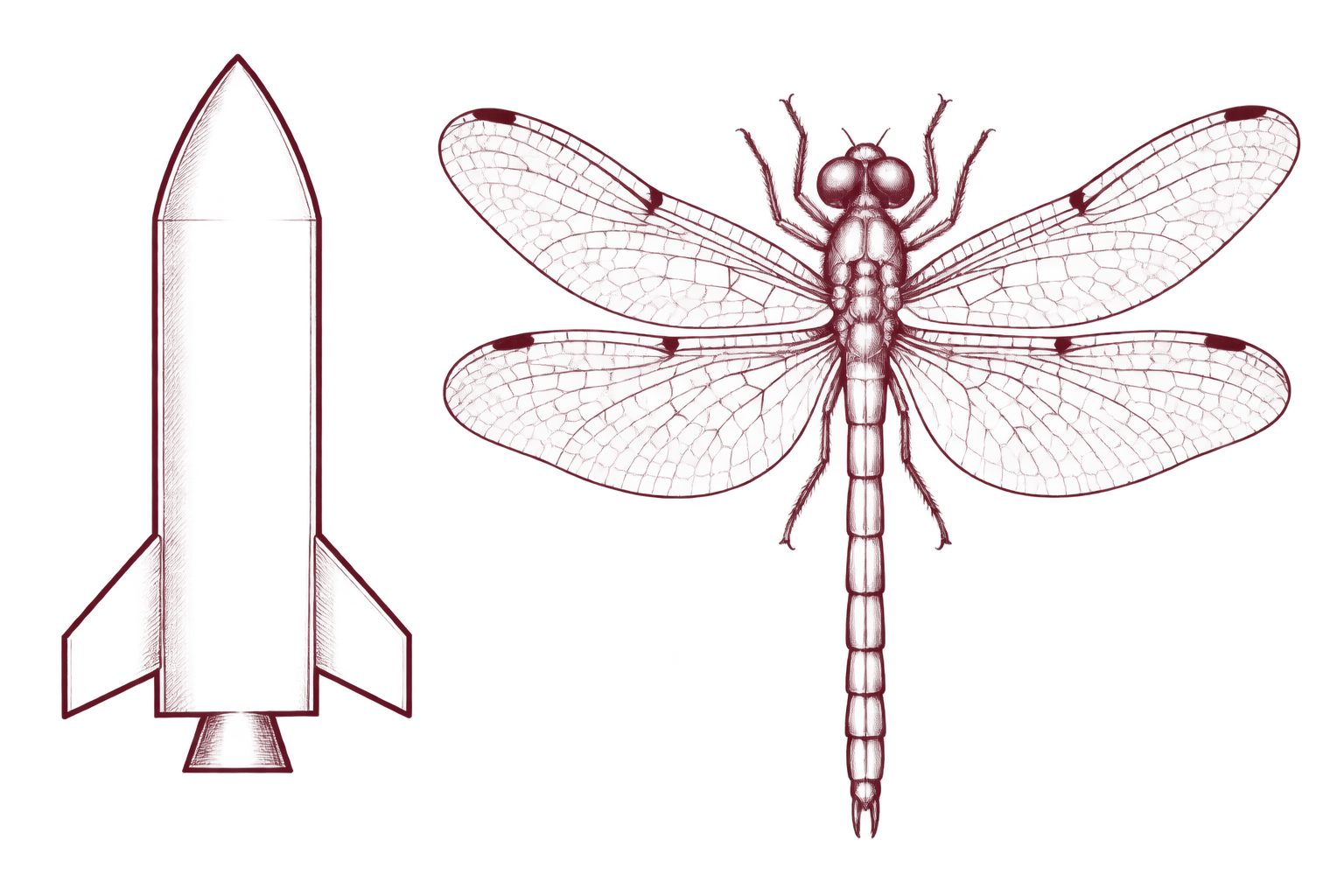
A rocket appears at the end of a moving chain of circles. At first there is barely a shape. Add more rotations, and a body emerges. Then fins. Then the outline becomes unmistakable.
My first reaction was simple: “this is super cool.” Then I started thinking about the process in reverse. Where did those circles come from? Who decided how long each arm should be, how quickly it should turn, and where it should start?
That is the part that blows my mind. You can begin with a drawing and calculate the motions needed to draw it back. The circles are not a trick someone carefully choreographed by hand. They are a different way of describing the path.
The rocket animation and dragonfly animation published by Philosophy Of Physics sparked this exploration. A machine made of rotations is a wonderful visual. But the deeper idea is the round trip: shape into numbers, numbers back into shape.
If we can imagine something clearly enough to trace it, we can build a mathematical model that draws it back.
There is an important boundary around that claim. A model of a rocket’s outline is not a model of its aerodynamics. A finite set of coefficients is an approximation of a continuous curve. But within that boundary, the result is remarkable: surprisingly simple ingredients can carry surprisingly intricate structure.
The drawing is the output. The spectrum is the recipe.
Think of a pen traveling around an outline. At every moment it has a horizontal position and a vertical position. Record those positions over time and you have two signals: x(t) and y(t).
Fourier analysis asks how much of each sine and cosine is present in those signals. The answer is a list of coefficients. Synthesis runs the process the other way: add those weighted waves, recover the coordinates, and put the pen there.
One rotation gives you a smooth, simple motion. More rotations add structure at progressively finer scales. Their speeds are related: one turn per cycle, two turns, three, and so on. Their lengths and starting angles carry the information specific to the drawing.
The recipe analogy works because a useful representation is executable. It does not merely label the picture “rocket.” It tells you how to produce positions along its outline. Change the recipe and you change the drawing in a predictable way.
That distinction matters. A photograph, a category name, and a path model can all describe the same object. Each makes different operations easy. Fourier coefficients make frequency-based editing easy: keep the broad motions, discard some fine detail, or inspect which scales dominate.
Watch a square emerge.
Before tackling fins or wing veins, start with a square. The drawing below is computed from coefficients, not a sequence of pre-rendered pictures. Move the control to see what survives when we keep fewer harmonics.
A concrete recipe for four corners
Take a square centered at the origin with side length two. Start at the lower-right corner, (1, −1), and travel counterclockwise at constant speed. One complete lap takes 2π units of time. That choice fixes the path, the starting point, the direction, and the speed.
A convenient construction begins with two triangular waves a quarter-cycle apart. Call them u(t) and v(t). Then set x = u + v and y = v − u. The resulting path visits (1, −1), (1, 1), (−1, 1), and (−1, −1), spending equal time on each edge.
u(t) = (8/π²) ∑k = 1, 3, 5, … cos(kt)/k²v(t) = u(t − π/2)
For this particular parameterization, only odd harmonics appear. Define Ak = 8/(π²k²) and sk = sin(kπ/2). The real coefficients are ax,k = Ak, bx,k = skAk, ay,k = −Ak, and by,k = skAk. Both coordinate means are zero.
The first five nonzero frequencies| Frequency k | Ak | sk |
|---|
| 1 | 0.81057 | +1 |
| 3 | 0.09006 | −1 |
| 5 | 0.03242 | +1 |
| 7 | 0.01654 | −1 |
| 9 | 0.01001 | +1 |
Keep only k = 1 and the pen draws a circle with radius about 1.146. At the starting corner it reaches approximately (0.811, −0.811), rather than (1, −1). Its distance from that corner is about 0.268. Higher odd frequencies progressively recover the straight edges and tighten the corners.
Notice the decay: these coefficients fall as 1/k². A square-shaped path has continuous coordinates; their slopes change abruptly at the corners. That differs from a square-wave signal, whose value jumps and whose coefficients fall as 1/k. The familiar persistent Gibbs overshoot belongs to those jumps. Here, the coordinates converge uniformly; corner rounding shrinks as we retain more terms. The derivative signals do have jumps.
Sharp features still ask more of a finite model. A broad curve is easy to recognize with a few slow motions. An abrupt turn needs faster motions to adjust the pen’s direction in a small part of the cycle.
Running the machine backward
To recover a Fourier model, first decide what the pen does. A visible outline is not yet a timed journey. Choose a starting point, an orientation, and a sampling rule. Uniform distance along the path is often a useful default because it avoids accidentally giving extra weight to places where a hand-drawn pen slowed down.
For a 2π-periodic coordinate, the standard real-series coefficient formulas are:
ak = (1/π) ∫02π x(t) cos(kt) dtbk = (1/π) ∫02π x(t) sin(kt) dt
Compute the same pair for y(t). The constant term supplies the mean position. Each integral measures alignment with one basis wave. Orthogonality lets us isolate one frequency without mixing it with the others; NIST’s Fourier-series reference gives the formal definitions and convergence conditions.
For a sampled drawing, we use a discrete Fourier transform. The FFT is an efficient way to calculate that transform. Keep every coefficient and the inverse transform recovers the sampled coordinates, within numerical precision. Keep fewer and you get an approximation. Exact recovery of the samples does not prove that unseen detail between samples was captured.
A small Python version of the reverse step
Provide evenly spaced samples in the chosen parameter, with no duplicate closing point. The function returns the mean and real-series coefficients for both coordinates. It excludes the special Nyquist bin to keep the reconstruction convention simple.
import numpy as np

def outline_to_real_coeffs(points, highest=9):
    p = np.asarray(points, dtype=float)
    if p.ndim != 2 or p.shape[1] != 2 or len(p) < 3:
        raise ValueError("Use at least three (x, y) samples")
    if not np.isfinite(p).all():
        raise ValueError("Coordinates must be finite")
    n = len(p)
    if not 1 <= highest <= (n - 1) // 2:
        raise ValueError("Highest frequency is out of range")
    spectrum = np.fft.rfft(p, axis=0) / n
    return (spectrum[0].real,
            2 * spectrum[1:highest + 1].real,
            -2 * spectrum[1:highest + 1].imag)

# At phase t, reconstruct the point with:
# mean + sum(a[k-1]*cos(k*t) + b[k-1]*sin(k*t))
# for k = 1 ... highest
The division by n matters: these coefficients assume NumPy’s default forward-transform normalization. See the NumPy rFFT documentation.
The route is part of the model
A dragonfly drawing makes this especially interesting. Its body and branching wing veins do not dictate one obvious continuous trip. A pen might trace the left wing first, return along a vein, cross the body, and trace the right. Another pen could visit the same lines in a different order.
The finished picture can look identical while the coordinate signals differ. So do the coefficients. Reverse direction and the frequency representation changes. Start elsewhere and phases change. Vary the speed and you redistribute structure across frequencies. Retracing a line counts as part of the journey even if it leaves no new visible ink.
This is a useful discipline for anyone building models: ask what was actually encoded. Here, the model represents a parameterized path, not a unique fingerprint of the static image. Multiple strokes may need separate paths, explicit pen lifts, or connecting segments that are omitted when rendering.
That is not a weakness of Fourier analysis. It is a reminder that representation begins with a choice. The data preparation is already part of the model.
Two views of the same motion
One visualization uses separate rotating assemblies for the horizontal and vertical coordinates. Project one onto x and the other onto y. Their guide lines meet at the pen. That arrangement makes the independence of the two coordinate signals easy to see.
Another puts everything into a single chain of rotating vectors. Write the point as the complex number z(t) = x(t) + iy(t). Euler’s formula turns each complex exponential into a rotation:
z(t) = ∑k ∈ ℤ ckeikt
Each coefficient determines a vector’s length and initial angle. Positive and negative frequencies turn in opposite directions. Add the vectors tip to tail and the last tip gives the position. The interactive above uses this view. 3Blue1Brown’s visual explanation is an excellent companion.
The two representations carry the same coordinate information. Each real coordinate has conjugate-symmetric Fourier coefficients; the combined complex path generally does not. That is why a single complex chain can need different clockwise and counterclockwise components.
What this teaches us about intelligent systems
The practical lesson is a design pattern: choose a representation, analyze the structure, retain what matters, reconstruct, and measure what changed. With the square, we can see the approximation error. In a larger system, we need equally explicit ways to test the result.
This connects directly to signal processing and transform-based compression. It also offers a precise neural-network example: Tancik and colleagues’ Fourier-feature work maps input coordinates through sinusoids to help networks learn high-frequency functions in low-dimensional domains. The model learns from a different representation of the inputs.
That does not mean a generative model is simply an epicycle machine, or that an agent reasons by running an FFT. The useful connection is more specific: a representation can make a difficult task easier, and reconstruction gives us something concrete to verify.
In agentic work, I care about that same loop. Can the system inspect something, build an explicit working model, make a controlled change, and check the result? Fourier drawing makes every stage visible. The coefficients are inspectable. The reconstruction is repeatable. The error can be measured against the original path.
Try the round trip.
Switch the demonstration to the rocket. Start with the lowest frequency and raise the limit. Watch which parts become recognizable first and which details arrive later. Then return to the square and compare the smooth edges with the corners.
For a deeper experiment, draw a closed outline of your own. Sample it, transform the coordinates, and reconstruct it with only a handful of frequencies. Repeat after changing the starting point or tracing speed. You will learn as much from the differences as from the likeness.
“If we can imagine it, we can model it” becomes useful when we add the next question: what exactly are we choosing to represent?
For this experiment, the answer is a path. And a path, translated into a spectrum, can become a drawing again. That is enough to change the way I look at a circle.
The spark behind this essay
Source animations & credits
The original videos were published by Philosophy Of Physics on Facebook. Both posts and their visible credits were reviewed on October 14, 2026. No individual creator is named in their captions.
- Rocket: Fourier reconstruction of an outline — two rotating chains reconstruct the horizontal and vertical coordinates, progressing from 1 to 100 harmonics per coordinate.
- Dragonfly: different routes, different coefficients — the post explains how changing the path through the wing veins changes the coefficients while preserving the drawing. It reports 8,192 harmonics per coordinate and a largest sampled deviation of about 0.14% of the dragonfly’s height; that is the publisher’s measurement, not an independent KUON benchmark.
Article by Mike Alford. The burgundy illustrations are new, AI-assisted KUON.ai interpretations inspired by those videos. The eight-second introduction builds simplified Fourier outlines, then reveals the illustrated detail; it does not reproduce the videos’ original coefficients or claim to reconstruct every engraved vein. The interactive reconstruction bench below the introduction computes its displayed curves directly from coefficients.
Mathematical references: NIST DLMF §1.8; Grant Sanderson / 3Blue1Brown, Fourier series; NumPy rFFT; Matthew Tancik and colleagues, Fourier Features.