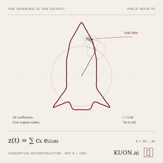
A chain of spinning circles draws a rocket. The mechanism looks absurdly complicated. The idea behind it is wonderfully simple.
In my first Fourier field note, I explored the round trip: trace an outline, turn its coordinates into coefficients, then use those coefficients to draw it back. This time I wanted to understand why the trick works.
The short answer is that the circles are not guessing. Each rotation contributes a precisely measured part of the original motion. Add those parts together and the pen follows the path.
First, turn the picture into a journey
An outline is not yet a signal. We have to choose where the pen starts, which way it travels, and how quickly it moves along each part of the curve.
Let one complete trip take a unit of time, from t = 0 to t = 1. The first article used a 2π-long cycle; this is the same mathematics with the time parameter rescaled. Now the pen has two signals: its horizontal position, x(t), and its vertical position, y(t). A closed path repeats, so both signals are periodic.
In a two-chain drawing, one chain supplies the horizontal coordinate and another supplies the vertical coordinate. Guide lines carry those two readings to their intersection: the pen. The chain endpoints do not have to touch each other. We are combining their coordinate readings, not physically joining the two mechanisms.
There is another perfectly valid arrangement: encode the whole path as z(t) = x(t) + iy(t). Then one chain of complex rotating vectors can place its endpoint directly on the outline. Same mathematics, different drawing apparatus.
One rotation is a building block
Euler’s formula gives us a compact description of a rotating unit vector:
Here k is an integer frequency: how many turns the vector makes during one trip around the drawing. Positive and negative frequencies turn in opposite directions. The zero-frequency term is a fixed offset, not a spinning arm.
Multiply that vector by a complex coefficient cₖ and we change its length and starting angle. Sum a collection of those weighted rotations and we get a much richer motion:
Use this for each coordinate separately, or for the complex path z(t). The coefficients carry the drawing. The circles make those coefficients visible.
Where the coefficients come from
This is the part I find most satisfying. We do not tune a thousand circles by hand. We calculate how much of each rotation is present in the chosen signal:
Think of the integral as a matching test. Multiply by the reverse of the frequency we are looking for, then average over a complete trip. The matching component stops rotating and survives the average. The others complete whole turns and cancel.
Mathematicians call that property orthogonality. Different integer-frequency rotations have zero average overlap over a full period. A frequency matches itself with an average of one.
That gives us more than an attractive animation. For a square-integrable periodic signal, these coefficients produce the unique best approximation, in mean-square error, among sums using the retained frequencies. This does not promise the smallest error at every individual point.
The circles are not a clever imitation of the drawing. They are an executable description of its motion.
What adding more circles actually improves
Low frequencies describe motion that changes slowly over the trip. Higher frequencies can correct changes happening in smaller intervals. Often that looks like a silhouette appearing first, followed by increasingly fine detail.
But frequency is not a ranking of importance. A small sharp feature may matter enormously to a human even if it contributes little to the total squared error. And the same outline, traversed at a different speed, has different coefficients.
For suitably smooth periodic coordinates, the coefficients decay quickly, so a modest set can work remarkably well. Under the usual piecewise-smooth conditions, Fourier sums converge to the coordinate value wherever it is continuous. At a jump, they converge to the midpoint of the two one-sided values. NIST’s Fourier-series reference gives the formal conditions.
A closed polygon needs one important distinction. Its position is continuous at a corner; its direction changes abruptly. The familiar persistent Gibbs overshoot belongs to a jump in a signal’s value. A corner is not automatically such a jump. For a constant-speed polygonal path, the coordinate coefficients decay as O(1/k²), and corner rounding shrinks as we retain more terms. The derivative signals do have jumps.
A thousand is a setting, not an accuracy guarantee
The note that started this article was labeled “N = 1000.” At that scale, a reconstruction can look almost indistinguishable from its target. But I would not attach a percentage to that impression without measuring it.
In the symmetric sum above, N is the highest retained positive frequency—not the total number of circles. Other visualizations use N to mean something else. A label alone cannot tell us how accurate a reconstruction is.
To make an accuracy claim, specify the path, the parameterization, the sampling method, and the error measure. Compare the original and reconstructed coordinates at matching parameter values. Report a root-mean-square error and, when the worst local miss matters, a maximum error too. Say what scale those numbers are normalized against.
There is a second boundary when working from sampled points. A discrete Fourier transform can recover those samples, within numerical precision, if we retain all its coefficients. It cannot prove that the sampling captured every detail of the original curve. Too few samples can alias distinct motions into the same data. The FFT makes the transform fast; it does not make missing information reappear. NumPy’s FFT documentation explains the discrete conventions.
The AI connection is representation, not magic
What interests me here is not a claim that neural networks are secretly Fourier drawing machines. They are not.
It is that changing the representation changes the work we can do. A list of pen positions is useful for replay. A spectrum makes it easier to inspect scales, remove selected frequencies, or compress a signal when most of its energy sits in relatively few coefficients. Filtering can help separate signal from noise when their frequency content differs; it is not a universal noise detector.
AI systems also depend on useful representations. Embeddings can make some similarities easier to compare. Learned features can expose patterns that are awkward to describe in raw inputs. But neural networks are not, in general, orthogonal basis expansions, and their features do not come with Fourier’s exact reconstruction guarantees.
That boundary matters. A representation earns its value through the operations it supports and the checks we can make—not through how impressive its output looks.
At KUON.ai, that is a useful standard for business systems built around agentic AI: what does the model preserve, what does it discard, and how do we check the result against the source? A convincing explanation is not the same as a verified one.
The spinning circles make that standard unusually easy to see. We can inspect the recipe, change it, run it, and compare the path it produces with the one we started from.
The wonder is still there. Now it has a reason.